Here are 10 steps to create a Wellington Boot from rotating circles (epicycles).
Ref 1: https://youtube.com/watch?v=qS4H6PEcCCA by
Ref 2: https://mathematica.stackexchange.com/questions/171755/how-can-i-draw-a-homer-with-epicycloids by anderstood for the code
Ref 3: Code file - if you need the code
Ref 4: The welly image
1) Create an account (14-day free trial available) at https://mathematica.wolframcloud.com
2) Create a new Wolfram notebook (File -> New Notebook)
Paste the following code into the top part of the notebook (takes a few seconds for Wolfram to recognise it):
img = Import["https://cdn.shopify.com/s/files/1/0001/1319/files/wellington-boot-black-and-white.gif?9529291750893159073"];
img = Binarize[img~ColorConvert~"Grayscale"];
img = ImageResize[img,100];
img = Blur[img,3];
pts = DeleteDuplicates@
Cases[Normal@
ListContourPlot[Reverse@ImageData[img],
Contours -> {0.5}], _Line, -1][[1, 1]];
center = Mean@MinMax[pts] & /@ Transpose@pts;
pts = # - center & /@ pts[[;; ;; 20]];
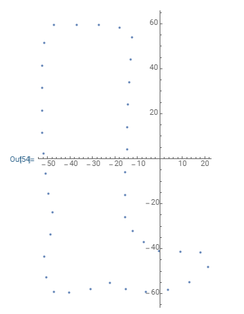
wellyPlot = ListPlot[pts, AspectRatio -> Automatic]
Note: You may need to adjust the ImageResize parameter above to a lower or higher number depending on the size of the input image.
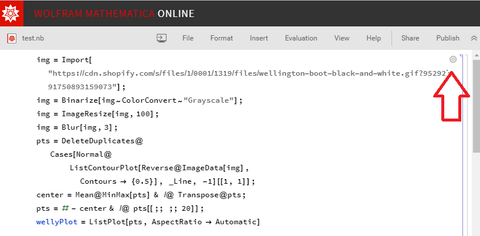
3) In the top-right corner click "Evaluate cell" (see red arrow in the diagram below)

4) Wait a few seconds for the code to evaluate
5) Paste the next block of code into the notebook below the plot
SetAttributes[toPt, Listable]
toPt[z_] := ComplexExpand[{Re@z, Im@z}] // Chop;
cf = Compile[{{z, _Complex, 1}},
Module[{n = Length@z},
1/n*Table[Sum[z[[k]]*Exp[-I*i*k*2 Pi/n], {k, 1, n}], {i, -m, m}]]];
z = pts[[All, 1]] + I*pts[[All, 2]];
m = 18;
cn = cf[z];
{f[t_], g[t_]} =
Sum[cn[[j]]*Exp[I*(j - m - 1)*t], {j, 1, 2 m + 1}] // toPt;
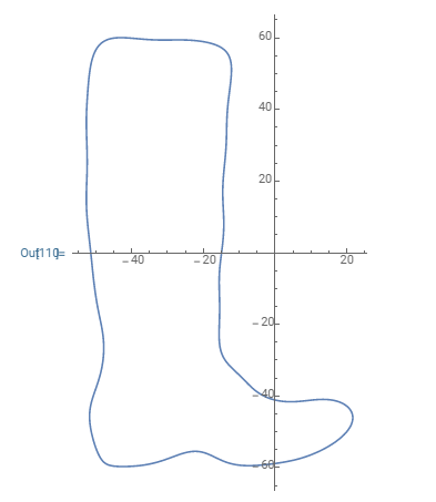
ParametricPlot[{f[t], g[t]}, {t, 0, 2 Pi}, AspectRatio -> Automatic]
Note: You may need to adjust the value of m above depending on the size of the image.
6) Click evaluate on the code
7) Wait for it to run
8) Paste the last code to animate the circles:
r = Abs /@ cn;
theta = Arg /@ cn;
index = {m + 1}~Join~
Riffle[Range[m + 2, 2 m + 1], Reverse[Range[1, m]]];
p[t_] = Accumulate@Table[cn[[j]]*Exp[I*(j - m - 1)*t], {j, index}] // toPt;
circles[t_] =
Table[Circle[p[t][[i]], r[[index[[i]]]]], {i, 1, 2 m + 1}];
anims = ParallelTable[
ParametricPlot[{f[s], g[s]}, {s, 0, t}, AspectRatio -> Automatic,
Epilog -> {circles[t][[2 ;;]], Line[p[t]], Point[p[t]]},
PlotRange -> {{-100, 50}, {-70, 60}}, ImageSize -> 400], {t, Subdivide[0.1, 4 Pi, 20]}];
ListAnimate@anims
Note: You may need to adjust the PlotRange x,y and x,y values to centre the plot.
9) And the result:
10) Let us know how you get along.


